Bird Audio Detection: baseline tests – and the problem of generalisation
Recently we launched the Bird Audio Detection Challenge, providing new datasets and a contest to improve the state of the art in general-purpose bird detection in audio.
So what is the state of the art? For a thorough answer, you can read our survey paper recently presented at the IEEE MLSP workshop 2016. For a numerical estimate of quality, we can take the data we’ve published, apply a couple of off-the-shelf methods, and see what happens…
An important thing we want to encourage through this challenge is generalisation. This means we want a detector that works across a wide range of species, and across a wide range of environments – without having to be manually tweaked each time it’s used in a different context. That’s why we published two very different datasets for you to develop your ideas on. One dataset is miscellaneous field recordings (containing birds about 25% of the time, and various other background sounds) from all around the world, while one is crowdsourced mobile-phone recordings from our bird classification app Warblr (containing birds about 75% of the time, and often with the sound of people mixed in) from all around the UK. (In the final test we’ll also have recordings from a site of high scientific interest: the Chernobyl Exclusion Zone.)
So here’s a question: if we take an existing machine-learning method, and “train” it using one of those datasets, can it generalise well enough to make sense of the other dataset?
We’ve looked at this question using two audio classifiers which we have here:
- The first is the classic “MFCCs and GMMs” method, which has been used in too many research papers to mention. It’s often a standard not-great baseline against which other methods are compared, but in some cases it may itself be good enough for the job. We used our open-source Python implementation of this called smacpy.
- The second is a variant of the method that we found useful for species classification: spherical k-means feature learning, followed by a Random Forest classifier. Described in more detail in our journal paper on large-scale classification of bird sounds. (Labelled as “skfl” in the plot below.)
So how well did they perform? Here’s a graph:
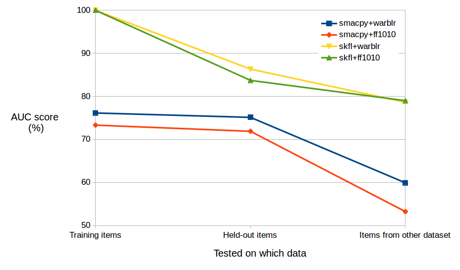
To understand the AUC value (Area Under the ROC Curve) on the y-axis: 100% is what we want, perfect detection, while 50% is the value you get for “pure ignorance” (e.g. flipping a coin to decide how to label each file).
The first thing you notice is that our “modern” classifier (in yellow and green) performs much better than the baseline MFCC+GMM classifier (orange and blue). OK, so far so good. In fact in the first column the modern classifier gets 100% performance – but that’s to be expected, since in the first column we test each system using the training data that it’s already seen.
Why doesn’t the MFCC+GMM classifier get 100% on the data it’s already seen? Essentially, it’s not powerful/flexible enough to create a map that fully captures all the yes/no decisions it has seen. So of course that’s showing a bit of a limitation. But when we look at the second column – testing the classifier using the same type of data as it was trained with, but using new unseen items – the “mediocre” performance continues at about the same level. The benefit of this inflexible classifier is that it has strongly avoided “overfitting” to any particular set of datapoints, even though it’s showing that it’s not great at the task.
The more powerful classifier does take a bit of a hit when we test it on unseen data – down from 100% to about 85%. I wouldn’t really have expected it to get 100% anyway, but you can see that if you’d only run the first test you might get a false impression…! Even though the performance goes down to 85% it is still stomping on the other classifier, outdoing it by a substantial margin.
This middle column is the kind of result you typically see quoted in research on classifiers. Train it on some data, test it on some similar-but-held-out data. But the third column is where it gets even more interesting!
In the third column, we test each classifier using data from the other dataset (warblr if we trained on ff1010; or ff1010 if we trained on warblr). Importantly, we’re still asking the same question (“Is there any bird or not?”), but the data represents different conditions under which we might ask that question. It certainly contains types of foreground and background sound that the classifier has never been exposed to during its training!
This is a test of generalisation, and you can see that the baseline MFCC+GMM classifier (“smacpy”) really falls at this hurdle. Its quality falls right down to 60% or lower (pretty close to the 50% of “perfect ignorance”!). The modern skfl classifier takes a bit of a hit too, falling to just below 80%. Not a major catastrophe, but below the performance we want to see for a general-purpose detector out in the field.
The two datasets represent related but different types of data collection scenario, and it’s not very surprising that a standard algorithm doesn’t know that we want it to generalise to those other related scenarios, not having been told anything about those other scenarios. In fact, a more “powerful” algorithm may often exhibit this issue more clearly, because it has the freedom to make use of the input data in all kinds of ways that might not be advisable! This issue has recently had a lot of attention in the “deep learning” field, where it has been found (among other things) that many different machine learning systems can be easily fooled by examples that lie outside the domain for which they were trained.
So what can we do about this? There are various techniques that might be useful, and in designing this challenge with bird audio we don’t want to pin things down about what approaches might work well. Maybe it’s possible to normalise the data, removing the factors that make the sound scenarios different from one another. Maybe it’s best not to lean too heavily on machine learning. Maybe it’s best to learn from existing work on how to build more generalisable systems. Maybe it’s best to use a few different methods and combine the results. In a future post we will go into this in more detail, outlining approaches that some researchers have been exploring.
If you’re developing a system to perform detection, the crucial thing to do is dig below the headline score. Don’t just look at the numbers. Find some examples that your system gets wrong (false positives and false negatives) and see if you can identify any tendencies that tell you why it’s doing what it’s doing.